


More on Economics & Investing

Desiree Peralta
3 years ago
How to Use the 2023 Recession to Grow Your Wealth Exponentially
This season's three best money moves.

“Millionaires are made in recessions.” — Time Capital
We're in a serious downturn, whether or not we're in a recession.
97% of business owners are decreasing costs by more than 10%, and all markets are down 30%.
If you know what you're doing and analyze the markets correctly, this is your chance to become a millionaire.
In any recession, there are always excellent possibilities to seize. Real estate, crypto, stocks, enterprises, etc.
What you do with your money could influence your future riches.
This article analyzes the three key markets, their circumstances for 2023, and how to profit from them.
Ways to make money on the stock market.
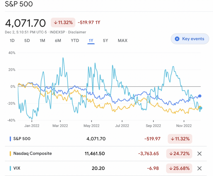
If you're conservative like me, you should invest in an index fund. Most of these funds are down 10-30% of ATH:
In earlier recessions, most money index funds lost 20%. After this downturn, they grew and passed the ATH in subsequent months.
Now is the greatest moment to invest in index funds to grow your money in a low-risk approach and make 20%.
If you want to be risky but wise, pick companies that will get better next year but are struggling now.
Even while we can't be 100% confident of a company's future performance, we know some are strong and will have a fantastic year.
Microsoft (down 22%), JPMorgan Chase (15.6%), Amazon (45%), and Disney (33.8%).
These firms give dividends, so you can earn passively while you wait.
So I consider that a good strategy to make wealth in the current stock market is to create two portfolios: one based on index funds to earn 10% to 20% profit when the corrections end, and the other based on individual stocks of popular and strong companies to earn 20%-30% return and dividends while you wait.
How to profit from the downturn in the real estate industry.
With rising mortgage rates, it's the worst moment to buy a home if you don't want to be eaten by banks. In the U.S., interest rates are double what they were three years ago, so buying now looks foolish.
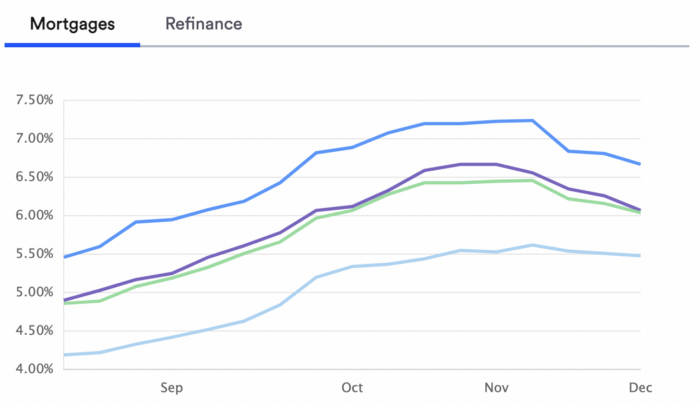
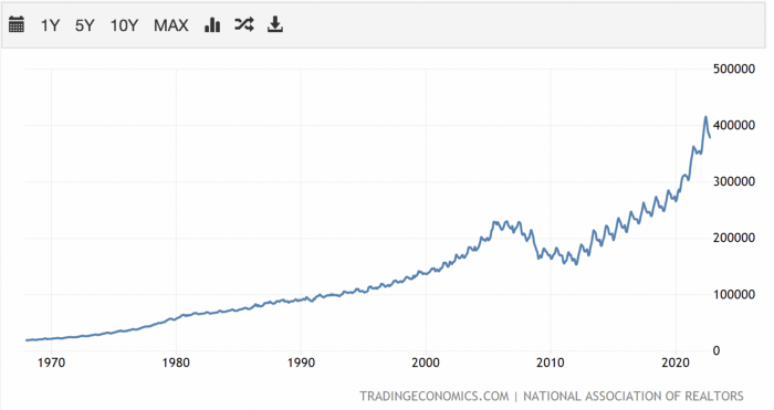
Due to these rates, property prices are falling, but that won't last long since individuals will take advantage.
According to historical data, now is the ideal moment to buy a house for the next five years and perhaps forever.
If you can buy a house, do it. You can refinance the interest at a lower rate with acceptable credit, but not the house price.
Take advantage of the housing market prices now because you won't find a decent deal when rates normalize.
How to profit from the cryptocurrency market.
This is the riskiest market to tackle right now, but it could offer the most opportunities if done appropriately.
The most powerful cryptocurrencies are down more than 60% from last year: $68,990 for BTC and $4,865 for ETH.
If you focus on those two coins, you can make 30%-60% without waiting for them to return to their ATH, and they're low enough to be a solid investment.
I don't encourage trying other altcoins because the crypto market is in crisis and you can lose everything if you're greedy.
Still, the main Cryptos are a good investment provided you store them in an external wallet and follow financial gurus' security advice.
Last thoughts
We can't anticipate a recession until it ends. We can't forecast a market or asset's lowest point, therefore waiting makes little sense.
If you want to develop your wealth, assess the money prospects on all the marketplaces and initiate long-term trades.
Many millionaires are made during recessions because they don't fear negative figures and use them to scale their money.

Ben Carlson
3 years ago
Bear market duration and how to invest during one
Bear markets don't last forever, but that's hard to remember. Jamie Cullen's illustration
A bear market is a 20% decline from peak to trough in stock prices.
The S&P 500 was down 24% from its January highs at its low point this year. Bear market.
The U.S. stock market has had 13 bear markets since WWII (including the current one). Previous 12 bear markets averaged –32.7% losses. From peak to trough, the stock market averaged 12 months. The average time from bottom to peak was 21 months.
In the past seven decades, a bear market roundtrip to breakeven has averaged less than three years.
Long-term averages can vary widely, as with all historical market data. Investors can learn from past market crashes.
Historical bear markets offer lessons.
Bear market duration
A bear market can cost investors money and time. Most of the pain comes from stock market declines, but bear markets can be long.
Here are the longest U.S. stock bear markets since World war 2:
Stock market crashes can make it difficult to break even. After the 2008 financial crisis, the stock market took 4.5 years to recover. After the dotcom bubble burst, it took seven years to break even.
The longer you're underwater in the market, the more suffering you'll experience, according to research. Suffering can lead to selling at the wrong time.
Bear markets require patience because stocks can take a long time to recover.
Stock crash recovery
Bear markets can end quickly. The Corona Crash in early 2020 is an example.
The S&P 500 fell 34% in 23 trading sessions, the fastest bear market from a high in 90 years. The entire crash lasted one month. Stocks broke even six months after bottoming. Stocks rose 100% from those lows in 15 months.
Seven bear markets have lasted two years or less since 1945.
The 2020 recovery was an outlier, but four other bear markets have made investors whole within 18 months.
During a bear market, you don't know if it will end quickly or feel like death by a thousand cuts.
Recessions vs. bear markets
Many people believe the U.S. economy is in or heading for a recession.
I agree. Four-decade high inflation. Since 1945, inflation has exceeded 5% nine times. Each inflationary spike caused a recession. Only slowing economic demand seems to stop price spikes.
This could happen again. Stocks seem to be pricing in a recession.
Recessions almost always cause a bear market, but a bear market doesn't always equal a recession. In 1946, the stock market fell 27% without a recession in sight. Without an economic slowdown, the stock market fell 22% in 1966. Black Monday in 1987 was the most famous stock market crash without a recession. Stocks fell 30% in less than a week. Many believed the stock market signaled a depression. The crash caused no slowdown.
Economic cycles are hard to predict. Even Wall Street makes mistakes.
Bears vs. bulls
Bear markets for U.S. stocks always end. Every stock market crash in U.S. history has been followed by new all-time highs.
How should investors view the recession? Investing risk is subjective.
You don't have as long to wait out a bear market if you're retired or nearing retirement. Diversification and liquidity help investors with limited time or income. Cash and short-term bonds drag down long-term returns but can ensure short-term spending.
Young people with years or decades ahead of them should view this bear market as an opportunity. Stock market crashes are good for net savers in the future. They let you buy cheap stocks with high dividend yields.
You need discipline, patience, and planning to buy stocks when it doesn't feel right.
Bear markets aren't fun because no one likes seeing their portfolio fall. But stock market downturns are a feature, not a bug. If stocks never crashed, they wouldn't offer such great long-term returns.

Quant Galore
3 years ago
I created BAW-IV Trading because I was short on money.
More retail traders means faster, more sophisticated, and more successful methods.
Tech specifications
Only requires a laptop and an internet connection.
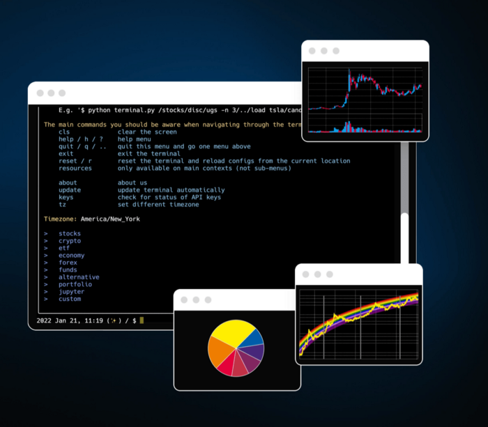
We'll use OpenBB's research platform for data/analysis.
Pricing and execution on Options-Quant

Background
You don't need to know the arithmetic details to use this method.
Black-Scholes is a popular option pricing model. It's best for pricing European options. European options are only exercisable at expiration, unlike American options. American options are always exercisable.
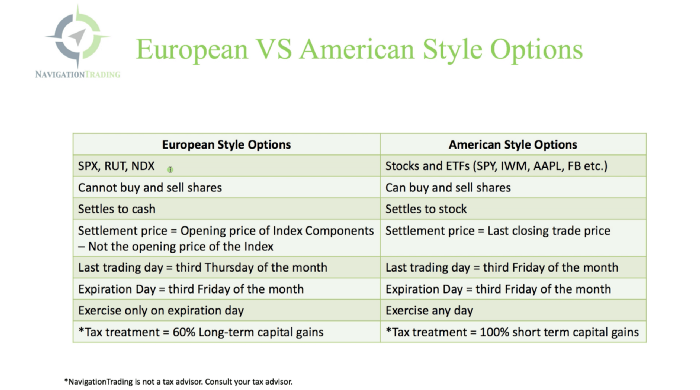
American options carry a premium to cover for the risk of early exercise. The Black-Scholes model doesn't account for this premium, hence it can't price genuine, traded American options.
Barone-Adesi-Whaley (BAW) model. BAW modifies Black-Scholes. It accounts for exercise risk premium and stock dividends. It adds the option's early exercise value to the Black-Scholes value.
The trader need not know the formulaic derivations of this model.
https://ir.nctu.edu.tw/bitstream/11536/14182/1/000264318900005.pdf
Strategy
This strategy targets implied volatility. First, we'll locate liquid options that expire within 30 days and have minimal implied volatility.
After selecting the option that meets the requirements, we price it to get the BAW implied volatility (we choose BAW because it's a more accurate Black-Scholes model). If estimated implied volatility is larger than market volatility, we'll capture the spread.
(Calculated IV — Market IV) = (Profit)
Some approaches to target implied volatility are pricey and inaccessible to individual investors. The best and most cost-effective alternative is to acquire a straddle and delta hedge. This may sound terrifying and pricey, but as shown below, it's much less so.
The Trade
First, we want to find our ideal option, so we use OpenBB terminal to screen for options that:
Have an IV at least 5% lower than the 20-day historical IV
Are no more than 5% out-of-the-money
Expire in less than 30 days
We query:
stocks/options/screen/set low_IV/scr --export Output.csv
This uses the screener function to screen for options that satisfy the above criteria, which we specify in the low IV preset (more on custom presets here). It then saves the matching results to a csv(Excel) file for viewing and analysis.
Stick to liquid names like SPY, AAPL, and QQQ since getting out of a position is just as crucial as getting in. Smaller, illiquid names have higher inefficiencies, which could restrict total profits.

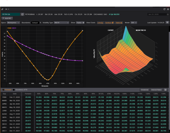
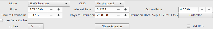
We calculate IV using the BAWbisection model (the bisection is a method of calculating IV, more can be found here.) We price the IV first.
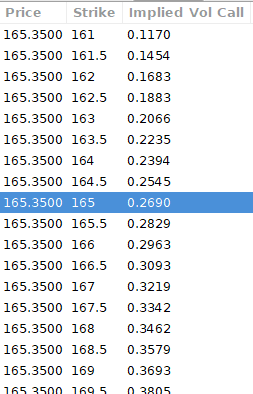
According to the BAW model, implied volatility at this level should be priced at 26.90%. When re-pricing the put, IV is 24.34%, up 3%.
Now it's evident. We must purchase the straddle (long the call and long the put) assuming the computed implied volatility is more appropriate and efficient than the market's. We just want to speculate on volatility, not price fluctuations, thus we delta hedge.
The Fun Starts
We buy both options for $7.65. (x100 multiplier). Initial delta is 2. For every dollar the stock price swings up or down, our position value moves $2.

We want delta to be 0 to avoid price vulnerability. A delta of 0 suggests our position's value won't change from underlying price changes. Being delta-hedged allows us to profit/lose from implied volatility. Shorting 2 shares makes us delta-neutral.
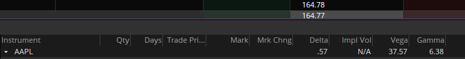
That's delta hedging. (Share price * shares traded) = $330.7 to become delta-neutral. You may have noted that delta is not truly 0.00. This is common since delta-hedging means getting as near to 0 as feasible, since it is rare for deltas to align at 0.00.
Now we're vulnerable to changes in Vega (and Gamma, but given we're dynamically hedging, it's not a big risk), or implied volatility. We wanted to gamble that the position's IV would climb by at least 2%, so we'll maintain it delta-hedged and watch IV.
Because the underlying moves continually, the option's delta moves continuously. A trader can short/long 5 AAPL shares at most. Paper trading lets you practice delta-hedging. Being quick-footed will help with this tactic.
Profit-Closing
As expected, implied volatility rose. By 10 minutes before market closure, the call's implied vol rose to 27% and the put's to 24%. This allowed us to sell the call for $4.95 and the put for $4.35, creating a profit of $165.

You may pull historical data to see how this trade performed. Note the implied volatility and pricing in the final options chain for August 5, 2022 (the position date).

Final Thoughts
Congratulations, that was a doozy. To reiterate, we identified tickers prone to increased implied volatility by screening OpenBB's low IV setting. We double-checked the IV by plugging the price into Options-BAW Quant's model. When volatility was off, we bought a straddle and delta-hedged it. Finally, implied volatility returned to a normal level, and we profited on the spread.
The retail trading space is very quickly catching up to that of institutions. Commissions and fees used to kill this method, but now they cost less than $5. Watching momentum, technical analysis, and now quantitative strategies evolve is intriguing.
I'm not linked with these sites and receive no financial benefit from my writing.
Tell me how your experience goes and how I helped; I love success tales.
You might also like

Maria Stepanova
3 years ago
How Elon Musk Picks Things Up Quicker Than Anyone Else
Adopt Elon Musk's learning strategy to succeed.

Medium writers rank first and second when you Google “Elon Musk's learning approach”.
My article idea seems unoriginal. Lol
Musk is brilliant.
No doubt here.
His name connotes success and intelligence.
He knows rocket science, engineering, AI, and solar power.
Musk is a Unicorn, but his skills aren't special.
How does he manage it?
Elon Musk has two learning rules that anyone may use.
You can apply these rules and become anyone you want.
You can become a rocket scientist or a surgeon. If you want, of course.
The learning process is key.
Make sure you are creating a Tree of Knowledge according to Rule #1.
Musk told Reddit how he learns:
“It is important to view knowledge as sort of a semantic tree — make sure you understand the fundamental principles, i.e. the trunk and big branches, before you get into the leaves/details or there is nothing for them to hang onto.”
Musk understands the essential ideas and mental models of each of his business sectors.
He starts with the tree's trunk, making sure he learns the basics before going on to branches and leaves.
We often act otherwise. We memorize small details without understanding how they relate to the whole. Our minds are stuffed with useless data.
Cramming isn't learning.
Start with the basics to learn faster. Before diving into minutiae, grasp the big picture.

Rule #2: You can't connect what you can't remember.
Elon Musk transformed industries this way. As his expertise grew, he connected branches and leaves from different trees.
Musk read two books a day as a child. He didn't specialize like most people. He gained from his multidisciplinary education. It helped him stand out and develop billion-dollar firms.
He gained skills in several domains and began connecting them. World-class performances resulted.
Most of us never learn the basics and only collect knowledge. We never really comprehend information, thus it's hard to apply it.
Learn the basics initially to maximize your chances of success. Then start learning.
Learn across fields and connect them.
This method enabled Elon Musk to enter and revolutionize a century-old industry.

Neeramitra Reddy
3 years ago
The best life advice I've ever heard could very well come from 50 Cent.
He built a $40M hip-hop empire from street drug dealing.
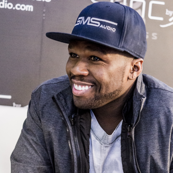
50 Cent was nearly killed by 9mm bullets.
Before 50 Cent, Curtis Jackson sold drugs.
He sold coke to worried addicts after being orphaned at 8.
Pursuing police. Murderous hustlers and gangs. Unwitting informers.
Despite his hard life, his hip-hop career was a success.
An assassination attempt ended his career at the start.
What sane producer would want to deal with a man entrenched in crime?
Most would have drowned in self-pity and drank themselves to death.
But 50 Cent isn't most people. Life on the streets had given him fearlessness.
“Having a brush with death, or being reminded in a dramatic way of the shortness of our lives, can have a positive, therapeutic effect. So it is best to make every moment count, to have a sense of urgency about life.” ― 50 Cent, The 50th Law
50 released a series of mixtapes that caught Eminem's attention and earned him a $50 million deal!
50 Cents turned death into life.
Things happen; that is life.
We want problems solved.
Every human has problems, whether it's Jeff Bezos swimming in his billions, Obama in his comfortable retirement home, or Dan Bilzerian with his hired bikini models.
All problems.
Problems churn through life. solve one, another appears.
It's harsh. Life's unfair. We can face reality or run from it.
The latter will worsen your issues.
“The firmer your grasp on reality, the more power you will have to alter it for your purposes.” — 50 Cent, The 50th Law
In a fantasy-obsessed world, 50 Cent loves reality.
Wish for better problem-solving skills rather than problem-free living.
Don't wish, work.
We All Have the True Power of Alchemy
Humans are arrogant enough to think the universe cares about them.
That things happen as if the universe notices our nanosecond existences.
Things simply happen. Period.
By changing our perspective, we can turn good things bad.
The alchemists' search for the philosopher's stone may have symbolized the ability to turn our lead-like perceptions into gold.
Negativity bias tints our perceptions.
Normal sparring broke your elbow? Rest and rethink your training. Fired? You can improve your skills and get a better job.
Consider Curtis if he had fallen into despair.
The legend we call 50 Cent wouldn’t have existed.
The Best Lesson in Life Ever?
Neither avoid nor fear your reality.
That simple sentence contains every self-help tip and life lesson on Earth.
When reality is all there is, why fear it? avoidance?
Or worse, fleeing?
To accept reality, we must eliminate the words should be, could be, wish it were, and hope it will be.
It is. Period.
Only by accepting reality's chaos can you shape your life.
“Behind me is infinite power. Before me is endless possibility, around me is boundless opportunity. My strength is mental, physical and spiritual.” — 50 Cent
Matthew Royse
3 years ago
5 Tips for Concise Writing
Here's how to be clear.
“I have only made this letter longer because I have not had the time to make it shorter.” — French mathematician, physicist, inventor, philosopher, and writer Blaise Pascal
Concise.
People want this. We tend to repeat ourselves and use unnecessary words.
Being vague frustrates readers. It focuses their limited attention span on figuring out what you're saying rather than your message.
Edit carefully.
“Examine every word you put on paper. You’ll find a surprising number that don’t serve any purpose.” — American writer, editor, literary critic, and teacher William Zinsser
How do you write succinctly?
Here are three ways to polish your writing.
1. Delete
Your readers will appreciate it if you delete unnecessary words. If a word or phrase is essential, keep it. Don't force it.
Many readers dislike bloated sentences. Ask yourself if cutting a word or phrase will change the meaning or dilute your message.
For example, you could say, “It’s absolutely essential that I attend this meeting today, so I know the final outcome.” It’s better to say, “It’s critical I attend the meeting today, so I know the results.”
Key takeaway
Delete actually, completely, just, full, kind of, really, and totally. Keep the necessary words, cut the rest.
2. Just Do It
Don't tell readers your plans. Your readers don't need to know your plans. Who are you?
Don't say, "I want to highlight our marketing's problems." Our marketing issues are A, B, and C. This cuts 5–7 words per sentence.
Keep your reader's attention on the essentials, not the fluff. What are you doing? You won't lose readers because you get to the point quickly and don't build up.
Key takeaway
Delete words that don't add to your message. Do something, don't tell readers you will.
3. Cut Overlap
You probably repeat yourself unintentionally. You may add redundant sentences when brainstorming. Read aloud to detect overlap.
Remove repetition from your writing. It's important to edit our writing and thinking to avoid repetition.
Key Takeaway
If you're repeating yourself, combine sentences to avoid overlap.
4. Simplify
Write as you would to family or friends. Communicate clearly. Don't use jargon. These words confuse readers.
Readers want specifics, not jargon. Write simply. Done.
Most adults read at 8th-grade level. Jargon and buzzwords make speech fluffy. This confuses readers who want simple language.
Key takeaway
Ensure all audiences can understand you. USA Today's 5th-grade reading level is intentional. They want everyone to understand.
5. Active voice
Subjects perform actions in active voice. When you write in passive voice, the subject receives the action.
For example, “the board of directors decided to vote on the topic” is an active voice, while “a decision to vote on the topic was made by the board of directors” is a passive voice.
Key takeaway
Active voice clarifies sentences. Active voice is simple and concise.
Bringing It All Together
Five tips help you write clearly. Delete, just do it, cut overlap, use simple language, and write in an active voice.
Clear writing is effective. It's okay to occasionally use unnecessary words or phrases. Realizing it is key. Check your writing.
Adding words costs.
Write more concisely. People will appreciate it and read your future articles, emails, and messages. Spending extra time will increase trust and influence.
“Not that the story need be long, but it will take a long while to make it short.” — Naturalist, essayist, poet, and philosopher Henry David Thoreau